...

Div
class grid-row grid-gap
Div class desktop:grid-col-6 Image Modified Div class desktop:grid-col-6 Figure 13. The RTPP triple line buffer logic (reproduced with permission from J. Histochem. Cytochem. [4], 1974). "The RTPP was designed to do 3x3 neighborhood image-processing in parallel in the GPP. Associated with the three lines is an effective Y dynamic address used to order the three lines as to (Y-1,Y,Y+1). In reading a raster line pattern into the triple line buffer, the oldest line must be replaced with the newest line. Similarly, the other two lines need to be adjusted as (Y-1,Y,Y+1) to (Y,Y+1,Y+2). By selecting the effective line address with a modulo three dynamic Y address counter, a dynamic Y address can be implemented. This is similar to the concept of buffer. The three X dynamic address vectors point to 3x3 neighborhood arrays in the line buffer. This neighborhood is called the current neighborhood. All of the dynamic address vectors are easily and efficiently programmed in the GPP to tessellate the current neighborhood along the three lines in the line buffer."

Image Modified

Anchor
Fig-RTPP-GPP-control-logic-FSM Fig-RTPP-GPP-control-logic-FSM

Figure 14. The RTPP GPP control logic finite state machine (reproduced with permission from J. Histochem. Cytochem. [4], 1974). "The GPP control logic is implemented as a finite state machine where the states of the system are defined from the logic flow of the system. This consists of the various bus, register enable and load signals. The state is a function of the current state and the current operator. Thus, to extend the machine, additional states and transitions between states would have been added (see [TR-7,TR-22])."

Image Modified

Anchor
Fig-RTPP-Examples-of-GPASM-code Fig-RTPP-Examples-of-GPASM-code

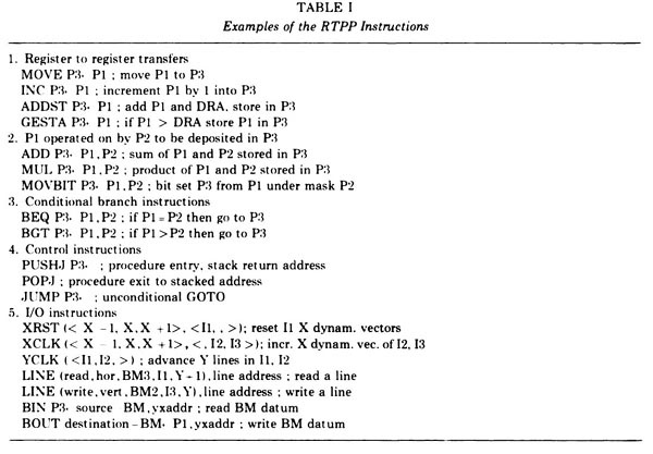
Figure 15. The Examples of RTPP instructions for the GPP (reproduced with permission from J. Histochem. Cytochem. [4], 1974). The Pi refers to a 3x3 pixel neighborhood that would be tessellated through the entire image. The GPP instructions [A HREF="#TR-22">TR-22] could be compiled by the GPPASM [A HREF="#TR-16">TR-16] assembler program running on the PDP8e and then loaded into the GPP instruction memory. A debugger for the GPP was DDTG that ran on the PDP8e [A HREF="#TR-2">TR-2] but controlled the GPP and buffer memories. We had also been evaluating collaborating on the construction of a MAINSAIL(R)  compiler to generate GPP assembly code so we could program the RTPP in a SAIL-like language.

...

Another of the projects Lew and I were also working on was the construction of a 3D brain atlas of an anolus lizard brain using aligned microtomed serial-section images. (Some of the goals for that project were similar to that of the National Library of Medicine's Visible Human. However, this was well before adequate computer technology and resources were available to implement such an atlas.) We wrote a PDP8e program to move the optical microscope stage in (X,Y) while keeping the center of the brain in the scanned visual center of the image field as we switched slides in a series of microtomed serial sections (the Z-axis control was not used in this operation). Each centered image could then be captured and saved as a disk file. The next section visible on the TV camera was compared with the image previously captured and stored in the image buffer memory. This procedure was iteratively repeated with subsequent slides to capture a sequence of aligned serial sections from a set of slides. The buffer memory data was saved at each point on 9-track magnetic tape. (This alignment software subsequently led to our involvement with 2D electrophoretic gels analysis [discussed below].) The set of serial sections could then be re-accessed sequentially to step through the brain slices centered at the selected point. We could generate movie loops with the BMON2 software to move virtually up and down through the serial sections at various frame rates. Because we could store sixteen 256x256 images in the buffer memory, the loops could have up to 16 sections and allowed us to visualize the 3D structure of part of the brain.

Image Modified

Anchor
Macrophage-with-Amosite-24Hr-phase-contrast Macrophage-with-Amosite-24Hr-phase-contrast

Figure 16. Photomicrograph of P388D1 macrophage-like cells 24 hours after amosite asbestos treatment used to study fiber-induced cytotoxicity [9] (reproduced with permission from Environmental Health Perspectives, 1980).

Image Modified

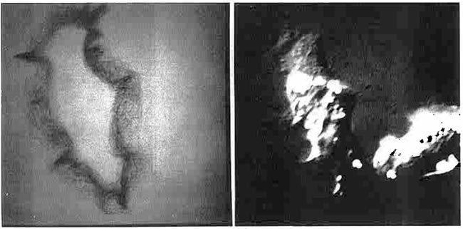
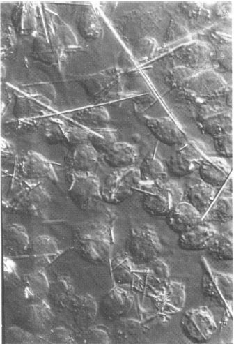
Figure 17. (Left) Boundary trace transform (BTT) of 233 images of 15-second interval scans of a single living P388D1 macrophage-like cell (left) (reproduced with permission from Environmental Health Perspectives, 1980 [9]). The boundaries for this set of images were traced by hand using a graphics tablet connected to the RTPP. The BTT is a 2D boundary frequency histogram where darker (higher frequency) pixels indicate boundaries of the cell that are more adherent to the glass slide and have less motility. BMON2 captured the set of images data and double buffered them to 9-track magnetic tape, with a 15-second image-sampling interval between scans. (Right) Illustration of a single cell captured by the RTPP using differential interference optics. The algorithm is described in several papers [8, 9]. Movies were made on the RTPP of a subsequence of 16 of the images in which you could see the cell trying to ingest the fiber, the fiber breaking through the other side of the cell (membrane), and then the cell backing up to try to reingest that part of the fiber, etc. These images allowed us to create a probability distribution of adhesion strength for boundary points of amoeboid cells. Points with low probability would flutter and extend. Looking at individual boundaries would not reveal this type of information; it was the ability to integrate large quantities of data that allowed these patterns to be detected. This was the way we thought the system should have been used - finding interesting results when no other method for doing so was possible.

...

The FLICKER software allowed users to measure spots as a set of (X,Y) image positions and integrated-densities for each sample. We manually recorded this data for later analysis, manually defining spots to be corresponding if they aligned well with FLICKER.

Image Modified

Anchor
lightBoxCameraStation lightBoxCameraStation

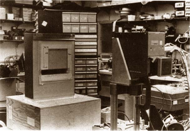
Figure 18. This was the alternative image acquisition setup. (Reproduced from a figure with permission from a reprint from Environmental Health Perspectives, 1980 [9].) A high-quality uniform illumination Aristo light box and Quantimet Vidicon TV camera were used for non-microscope images. A gel autoradiograph, wet 2D gel, electron micrograph, or other transparent sample object was placed on the light box and scanned using the RTPP/Vidicon camera. A NBS standard neutral density step wedge was placed on the bottom of the scan area. This was captured along with the image and was used to calibrate the grayscale pixel data to optical density using a piecewise linear curve fitting algorithm (see [9] for an example). As an aside, the electronics workbench area in the background was where many of the local RTPP electronics assembly was performed in the Park Building.

...